%pylab inline
from IPython.display import Image

Populating the interactive namespace from numpy and matplotlib

Quick introduction of the idea

Convolutional-type Constraint

Our goal is to construct a density field realization \(f(\mathbf x)\) subject to a set of \(M\) constraints:

\[\Gamma = \{ C_i \equiv C_i [f; \mathbf r_c] = c_i; i = 1,...,M \}\]

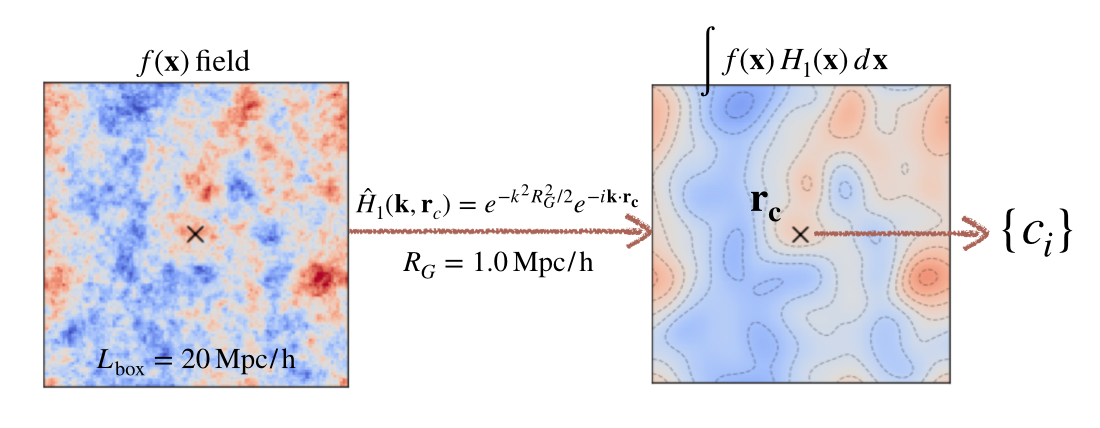
The constraint \(C_i[f;\mathbf r_c]\) can be viewed as a functional of the \(f(\mathbf x)\) field to have specific value \(c_i\) at position \(\mathbf x = \mathbf r_c\). We only consider linear functionals of the field, that the constraint value \(c_i\) is obtained by convolving the \(f(\mathbf x)\) field with some kernel \(H_i(\mathbf x, \mathbf r_c)\) leading to the convolved field value at position \(\mathbf r_c\). We can write \(C_i\) in the form of:

\[C_i[f;\mathbf r_c] = \int d\mathbf{x} f(\mathbf x) H_i(\mathbf x, \mathbf r_c) = \int \frac{d \mathbf{k}} {(2 \pi)^3} \hat{f}(\mathbf k) H^{*}_i (\mathbf k, \mathbf r_c) = c_i\]

As an simple example below, we convolve the linear density field (2D projection) with a simple Gaussian kernel of width 1 Mpc/h and aim to constrain/specify the convolved value at center \(\mathbf r_c\) to be \(c_i\)

Image(filename='convolve.png', width=600)

Ensemble Mean Field \(\bar{f}_{\Gamma}(\mathbf x)\)

Given a certain constraint set \(\Gamma\), one can build a corresponding “ensemble mean field” via:

\[\bar{f_{\Gamma}}(\mathbf x) \equiv <f(\mathbf x)|\Gamma> = \xi_i(\mathbf x) \xi^{-1}_{ij} c_j\]

where \(\xi_i(\mathbf x) = <f(\mathbf x)C_i[f;\mathbf r_c]>\) is the average of the cross-correlation between the \(f(\mathbf x)\) field and the \(i\)th constraint \(C_i\), and \(\xi^{-1}_{ij}\) is the (\(ij\)) th element of the inverse of constraint’s covariance matrix \(<C_i C_j>\).

Using the definition of the matter power spectrum \(P(k)\),

\[(2\pi)^3 P(k_1) \delta_D(\mathbf k_1 - \mathbf k_2) = <\hat{f}(\mathbf k_1) \hat{f}^{*}(\mathbf k_2)>\]

we can write down the formalism for \(\xi_i(\mathbf x)\) and \(\xi_{ij}\) as follows:

\begin{equation}\label{equation:xi_i} \begin{split} \xi_i(\mathbf x) & \equiv <f(\mathbf x) C_i[f;\mathbf r_c]> \\ & = <\int \frac{d \mathbf{k_1}} {(2 \pi)^3} \hat{f}(\mathbf k_1) e^{i \mathbf k_1 \cdot \mathbf x} \int \frac{d \mathbf{k_2}} {(2 \pi)^3} \hat{f}^{*}(\mathbf k_2) H_i (\mathbf k_2,\mathbf r_c)> \\ &= \int \frac{d \mathbf{k_1}} {(2 \pi)^3} \frac{d \mathbf{k_2}} {(2 \pi)^3} <\hat{f}(\mathbf k_1) \hat{f}^{*}(\mathbf k_2)> H_i (\mathbf k_2, \mathbf r_c) e^{i \mathbf k_1 \cdot \mathbf x} \\ &= \int \frac{d \mathbf{k}} {(2 \pi)^3} P(k) \hat{H}_i(\mathbf k, \mathbf r_c) e^{i \mathbf{k} \cdot \mathbf x} \end{split} \end{equation}

and

\begin{equation}\label{equation:xi_ij} \begin{split} \xi_{ij} & \equiv <C_i[f;\mathbf r_c] C_j[f;\mathbf r_c]> \\ &= <\int \frac{d \mathbf{k_1}} {(2 \pi)^3} \hat{f}(\mathbf k_1) H^{*}_i (\mathbf k_1, \mathbf r_c) \int \frac{d \mathbf{k_2}} {(2 \pi)^3} \hat{f^*}(\mathbf k_2) H_j (\mathbf k_2, \mathbf r_c)> \\ &= \int \frac{d \mathbf{k}} {(2 \pi)^3} \hat{H}^{*}_i (\mathbf k, \mathbf r_c) \hat{H}_j (\mathbf k, \mathbf r_c) P(k) \end{split} \end{equation}

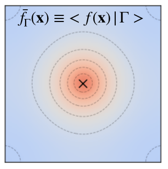
Intuitively, the ensemble mean field \(\bar{f_{\Gamma}}(\mathbf x)\) can be interpreted as the “most likely” field subject to the set of constraints \(\Gamma\).

For example, the field shown below is the ensemble mean field corresponding to a 3\(\sigma_0\) peak at the center of the box:

Image(filename='ensemble-mean.png', width=180)

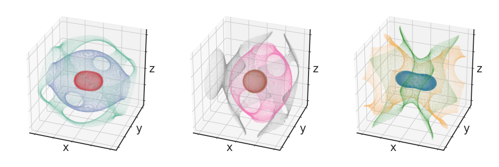
With a combination of different types of constraints \(C_i\) (with kernel \(H_i(\mathbf k)\)), we can construct ensemble mean field that specifies the shape (left plot), peculiar velocity (middle) and tidal field (right) at the site of the peak. See Build_Ensemble_Mean_Field in the tutorial for further details.

Image(filename='contour3D-ensemble.png', width=600)
# a 3D illustration of the ensemble mean field constructed via different constraints

Construct a constrained realization

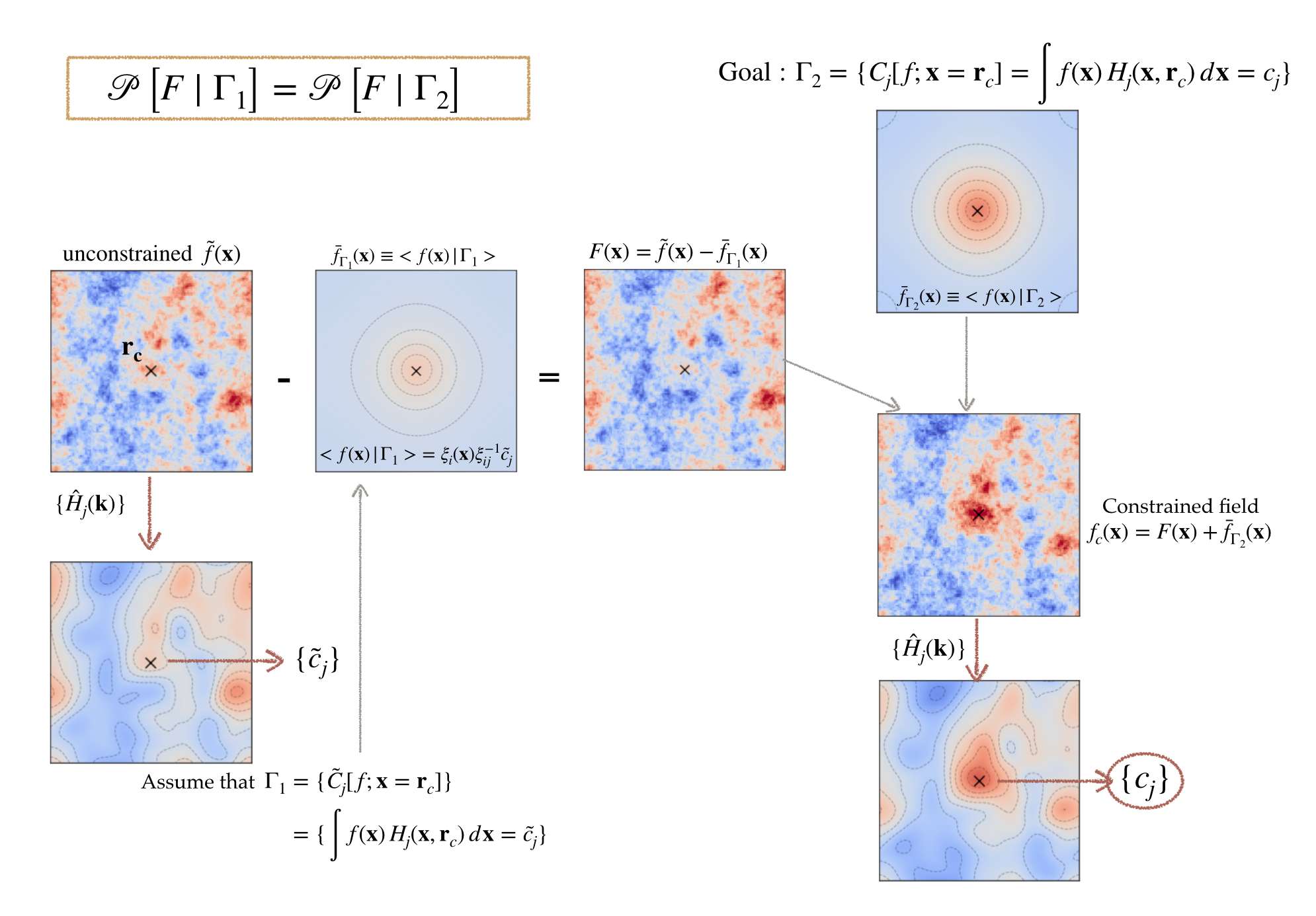
The CR formalism further introduces the “residual field” \(F(\mathbf x) \equiv f(\mathbf x) - \bar{f_{\Gamma}}(\mathbf x)\) as the difference between an arbitrary Gaussian realization \(f(\mathbf x)\) satisfying the constraint set \(\Gamma\) and the ensemble mean field \(\bar{f_{\Gamma}}(\mathbf x)\) of all those fields. The crucial idea behind the CR construction method is based on the fact that, the complete probability distribution \(\mathscr{P} [F|\Gamma]\) of the residual field \(F(\mathbf x)\) is independent of the numerical values \(c_i\) of the constraints \(\Gamma\).

i.e., for any \(\Gamma_1\), \(\Gamma_2\), we have

\begin{equation} \mathscr{P} [F|\Gamma_1] = \mathscr{P} [F|\Gamma_2] \end{equation}

Therefore, one can construct the desired realization under constraint sets \(\Gamma\) by properly sampling a residual field \(F(\mathbf x)\) from a random, unconstrained realization \(\tilde{f} (\mathbf x)\) and then adding that \(F(\mathbf x)\) to the ensemble field \(\bar{f_{\Gamma}}(\mathbf x)\) corresponding to \(\Gamma\).

The formalism can be written as:

\begin{equation} \label{equation:construct_fx} \begin{split} f(\mathbf x) & = F(\mathbf x) + \bar{f}_{\Gamma}(\mathbf x) \\ &= (\tilde{f} (\mathbf x) - \bar{f}_{\tilde{\Gamma}}(\mathbf x)) + \bar{f}_{\Gamma}(\mathbf x) \\ &= (\tilde{f} (\mathbf x) - \xi_i(\mathbf x) \xi^{-1}_{ij} \tilde{c}_j) + \xi_i(\mathbf x) \xi^{-1}_{ij} c_j \\ &= \tilde{f} (\mathbf x) + \xi_i(\mathbf x) \xi^{-1}_{ij} (c_j - \tilde{c}_j) \end{split} \end{equation}

i.e., we are treating the original \(\tilde{f}(\mathbf x)\) as a field subject to constraint sets \(\tilde{\Gamma}\) with value \(\tilde{c}_j = C_j [\tilde{f}; \mathbf r_c]\), (\(\tilde{c}_j\) is the original value of the unconstrained field), and \(\bar{f}_{\tilde{\Gamma}}(\mathbf x) = \xi_i(\mathbf x) \xi^{-1}_{ij} \tilde{c}_j\) is the ensemble mean field corresponding to \(\tilde{\Gamma}\). From \(\tilde{f}(\mathbf x) - \bar{f}_{\tilde{\Gamma}}(\mathbf x)\) we get the residual field \(F(\mathbf x)\) from a random unconstrained realization, and adding that to \(\bar{f}_{\Gamma}(\mathbf x)\) results in the field \(f(\mathbf x)\) satisfying constraint \(\Gamma\).

Below is an illustration of the procedure:

Image(filename='apply-constraint.png', width=900)