Build Ensemble Mean Field¶

In this section, we show examples of how to use gsCR to build the Ensemble mean field subject to desired constraints.

Remind that the Ensemble mean field is built with \(\bar{f}(\mathbf x) = <f(\mathbf x)|\Gamma> = \xi_i(\mathbf x) \xi^{-1}_{ij} c_j\):

[1]:

%pylab inline

from gaussianCR.construct import *
from gaussianCR.cosmo import *
from gaussianCR.transform import *

Populating the interactive namespace from numpy and matplotlib

[2]:

# some style of the notebook
plt.rc('xtick', labelsize=15)
plt.rc('ytick', labelsize=15)
np.set_printoptions(precision=3,linewidth=150,suppress=True)

initialize cosmology

[3]:

import nbodykit.cosmology as nbcosmos
wmap9 = Cosmos(FLRW=True,obj=nbcosmos.WMAP9)

initialize gsCR object

Here we use wmap9 cosmology, set the box size to be 20 Mpc/\(h\), Gaussian kernel length \(R_G = 0.9\) Mpc/\(h\), density field in shape of (128,128,128)

[4]:

fg = gsCR(wmap9,Lbox=20,Nmesh=128,RG=0.9)

[5]:

print (fg)

  This is a gsCR object:
  Lbox = 20.0 Mpc/h
  Nmesh = 128
  RG = 0.9 Mpc/h
  Sigma0_RG = 1.82, Sigma2_RG = 1.78
  xpk = [0, 0, 0]
  CONS = ['full']
  xij_tensor_inv =
 None

Example 1: Shape of the peak

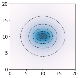
We build an ensemble mean field of a density peak in the center of the box, with constraints only imposed on the immediate surrounding of the peak with CONS = [‘f0’, ‘f2’]

We set peak height \(\nu = 4\sigma_0(R_G)\), compactness \(x_d = 3\sigma_2(R_G)\), axial ratio \((a_1/a_2)^2 = 2\), and \(\alpha_1 = \beta_1 = \phi_1 = 0\) so that \(a_1\) aligns along \(x\) axis.

[6]:

fg.xpk = [10,10,10]
fg.CONS = ['f0','f2']
fg.build_Xij_inv_matrix() # this need to be call whenever CONS is changed, to construct the covariance matrix

c_values = fg.set_c_values(nu=4,xd=3,a12sq=2) # set constraint values
dx_ensemble = fg.Ensemble_field(c_values)

Constrain peak parameters:
f0:  nu = 4.0 $\sigma_0$
f2:  xd = 3.0 $\sigma_2$, a12sq = 2.0, a13sq = 1.0,a1=0.00, b1=0.00, p1=0.00

We visualization of the ensemble mean field by projecting it to the xy plane

[7]:

den_field = np.transpose(np.sum(dx_ensemble,axis=-1))
plt.imshow(den_field,cmap="PuBu",origin='lower',alpha=0.8,extent=(0,fg.attrs['Lbox'],0,fg.attrs['Lbox']))
plt.contour(den_field,colors='black',alpha=0.8,linewidths=1,linestyles='dashed',levels=5,extent=(0,fg.attrs['Lbox'],0,fg.attrs['Lbox']))

[7]:

<matplotlib.contour.QuadContourSet at 0x7f15339b0e50>

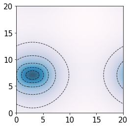
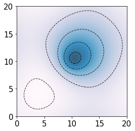
../_images/examples_Build_Ensemble_Mean_Field_11_1.png

We can quickly move the peak to the corner by directly updating xpk:

[8]:

fg.xpk = [3,7,10]
dx_ensemble = fg.Ensemble_field(c_values)

den_field = np.transpose(np.sum(dx_ensemble,axis=-1))
plt.imshow(den_field,cmap="PuBu",origin='lower',alpha=0.8,extent=(0,fg.attrs['Lbox'],0,fg.attrs['Lbox']))
plt.contour(den_field,colors='black',alpha=0.8,linewidths=1,linestyles='dashed',levels=5,extent=(0,fg.attrs['Lbox'],0,fg.attrs['Lbox']))

[8]:

<matplotlib.contour.QuadContourSet at 0x7f14e41f3a90>

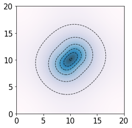
../_images/examples_Build_Ensemble_Mean_Field_13_1.png

We can make the peak more elliptical by setting axial ratio \((a_1/a_2)^2 = 3\), orienate the peak along (+1,+1,0) direction by setting \(\alpha_1 = 0.25 \pi\).

[9]:

fg.xpk = [10,10,10]
c_values = fg.set_c_values(nu=4,xd=3,a12sq=3,a1=0.25*np.pi) # set constraint values
dx_ensemble = fg.Ensemble_field(c_values)

den_field = np.transpose(np.sum(dx_ensemble,axis=-1))
plt.imshow(den_field,cmap="PuBu",origin='lower',alpha=0.8,extent=(0,fg.attrs['Lbox'],0,fg.attrs['Lbox']))
plt.contour(den_field,colors='black',alpha=0.8,linewidths=1,linestyles='dashed',levels=5,extent=(0,fg.attrs['Lbox'],0,fg.attrs['Lbox']))

Constrain peak parameters:
f0:  nu = 4.0 $\sigma_0$
f2:  xd = 3.0 $\sigma_2$, a12sq = 3.0, a13sq = 1.0,a1=0.79, b1=0.00, p1=0.00

[9]:

<matplotlib.contour.QuadContourSet at 0x7f1533efa950>

../_images/examples_Build_Ensemble_Mean_Field_15_2.png

Note on orientation:

The \(\alpha_1\), \(\beta_1\), \(\phi_1\) are the Euler angles that sets the rotational transformation of the principal axes of the mass ellipsoid. The rotational matrix is in ZX’Z’’ sequence, see https://mathworld.wolfram.com/EulerAngles.html

We can also know the direction of the peak by looking at gaussianCR.transform.set_Aij(a1,b1,p1)

e.g. in the above example, run set_Aij(a=0.25*np.pi,b=0,p=0):

array([[ 0.707,  0.707,  0.   ],  <--- direction of a1
       [-0.707,  0.707,  0.   ],  <--- direction of a2
       [ 0.   , -0.   ,  1.   ]]) <--- direction of a3

Example 2: peculiar velocity of the peak

Ensemble mean field of a density peak with peculiar velocity on scale of \(R_G\).

Here we set peak height \(\nu = 3\sigma_0(R_G)\), and peculiar velocity \(v_{G,x} = 60\) km/s in \(+x\) direction.

[10]:

fg.xpk=np.array([10,10,10])
fg.CONS = ['f0','vx']
fg.build_Xij_inv_matrix()
c_values = fg.set_c_values(nu=3,vx=60)

dx_ensemble = fg.Ensemble_field(c_values)
den_field = np.transpose(np.sum(dx_ensemble,axis=-1))
plt.imshow(den_field,cmap="PuBu",origin='lower',alpha=0.8,extent=(0,fg.attrs['Lbox'],0,fg.attrs['Lbox']))
plt.contour(den_field,colors='black',alpha=0.8,linewidths=1,linestyles='dashed',levels=5,extent=(0,fg.attrs['Lbox'],0,fg.attrs['Lbox']))

Constrain peak parameters:
f0:  nu = 3.0 $\sigma_0$
vx = 60.0 km/s

[10]:

<matplotlib.contour.QuadContourSet at 0x7f14e40e1390>

../_images/examples_Build_Ensemble_Mean_Field_18_2.png

Note that the peculiar velocity of the peak is induced by the overdensity of matter distribution to the right of the peak, therefore in positive \(x\) direction.

We can set density peak has \(v_{G,x} = v_{G,y} = 60\) km/s in both \(x\) and \(y\) direction:

[11]:

fg.xpk=np.array([10,10,10])
fg.CONS = ['f0','vx','vy']
fg.build_Xij_inv_matrix()
c_values = fg.set_c_values(nu=3,vx=60,vy=60)

dx_ensemble = fg.Ensemble_field(c_values)
den_field = np.transpose(np.sum(dx_ensemble,axis=-1))
plt.imshow(den_field,cmap="PuBu",origin='lower',alpha=0.8,extent=(0,fg.attrs['Lbox'],0,fg.attrs['Lbox']))
plt.contour(den_field,colors='black',alpha=0.8,linewidths=1,linestyles='dashed',levels=5,extent=(0,fg.attrs['Lbox'],0,fg.attrs['Lbox']))

Constrain peak parameters:
f0:  nu = 3.0 $\sigma_0$
vx = 60.0 km/s
vy = 60.0 km/s

[11]:

<matplotlib.contour.QuadContourSet at 0x7f14e4053290>

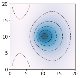
../_images/examples_Build_Ensemble_Mean_Field_20_2.png

Example 3: Tidal field around the peak

Ensemble mean field of a density peak with subject to the tidal field. Here we set peak height \(\nu = 4\sigma_0(R_G)\), with shear magnitude \(\epsilon=60\), shear angle \(\omega = 1.5\pi\), such that tidal field is (+30, -30, 0) km/s/Mpc in the three principal axes. We set the orientation of the tidal field \(\alpha_2 = \pi\), \(\beta_2 = 0\), \(\phi = 0.5 \pi\) (default setting), such that the peak is elongated in \(x\) direction and compressed in \(y\) direction.

[12]:

fg.xpk=np.array([10,10,10])
fg.CONS = ['f0','TG']
fg.build_Xij_inv_matrix()
c_values = fg.set_c_values(nu=4,epsilon=60,omega=1.5*np.pi)

dx_ensemble = fg.Ensemble_field(c_values)
den_field = np.transpose(np.sum(dx_ensemble,axis=-1))
plt.imshow(den_field,cmap="PuBu",origin='lower',alpha=0.8,extent=(0,fg.attrs['Lbox'],0,fg.attrs['Lbox']))
plt.contour(den_field,colors='black',alpha=0.8,linewidths=1,linestyles='dashed',levels=5,extent=(0,fg.attrs['Lbox'],0,fg.attrs['Lbox']))

Constrain peak parameters:
f0:  nu = 4.0 $\sigma_0$
TG:  epsilon = 60.0 km/s/Mpc, omega = 4.71, a2=3.14, b2=0.00, p2=1.57

[12]:

<matplotlib.contour.QuadContourSet at 0x7f14e4037c50>

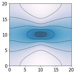
../_images/examples_Build_Ensemble_Mean_Field_22_2.png

Note on orientation:

We can set the direction of the tidal field by looking at gaussianCR.transform.set_Aij(a2,b2,p2)

e.g. in the above example, run set_Aij(a=np.pi,b=0,p=0.5*np.pi):

array([[-0., -1.,  0.],   <--- direction of smallest (negative) eigenvalue of Tij, compression
       [ 1., -0.,  0.],   <--- direction of largest (positive) eigenvalue of Tij, elongation
       [ 0.,  0.,  1.]])