Construct constrained realization

In this section, we show an example to use gsCR to constrain a random realization of linear density field. In this example, we use fastpm package to generate random realization of density field (at z=0).

%pylab inline

from pmesh.pm import ParticleMesh
from fastpm.core import leapfrog, Solver, autostages

from gaussianCR.construct import *
from gaussianCR.cosmo import *

Populating the interactive namespace from numpy and matplotlib

# some style of the notebook
plt.rc('xtick', labelsize=15)
plt.rc('ytick', labelsize=15)
np.set_printoptions(precision=3,linewidth=150,suppress=True)

---

initialize cosmology

import nbodykit.cosmology as nbcosmos
wmap9 = Cosmos(FLRW=True,obj=nbcosmos.WMAP9)

---

initialize gsCR object

Here we use wmap9 cosmology, set the box size to be 20 Mpc/\(h\), Gaussian kernel length \(R_G = 0.9\) Mpc/\(h\), density field in shape of (128,128,128)

Lbox = 20 # Mpc/h
Ng = 128  # number of grid to represent the dx_field
RG = 0.9  # Mpc/h

fg = gsCR(wmap9,Lbox,Ng,RG)

---

generate a random linear density field

Here we use fastpm and pmesh to generate a random realization of the linear density field with WMAP9 cosmology, with a random seed. Users can also import their own density field with the matched boxsize, shape and normalization. Note that our dx_field is the density contrast field \(\delta_x = \delta/\bar{\delta} - 1\) at \(z=0\).

pm = ParticleMesh(BoxSize=Lbox, Nmesh=[Ng,Ng,Ng])
Q = pm.generate_uniform_particle_grid(shift=0)
solver = Solver(pm,nbcosmos.WMAP9, B=1)

wn = solver.whitenoise(seed = 189953)
dlin = solver.linear(wn, lambda k: wmap9.Pk_lin(k))

# extract the linear field as a numpy array
dx_field = dlin.c2r().value

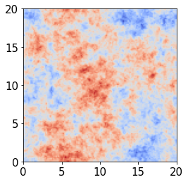
Let’s quickly visualize the random realization by projecting it on xy plane:

den_field = np.transpose(np.sum(dx_field,axis=-1))
plt.imshow(den_field,cmap='coolwarm',origin='lower',extent=(0,Lbox,0,Lbox))

<matplotlib.image.AxesImage at 0x7f3ca02e2ed0>

---

decide the position to impose the constraint

We can choose whereever we like to impose our constraints. One choice is to find the original peak of the linear density field. gsCR.find_xpk method would convolve dx_field with Gaussian kernel with scale \(R_G\) and find the peak of the smoothed dx_field.

xpk = fg.find_xpk(dx_field)
print (xpk)

fg.xpk = xpk

[10.156  8.594 13.438]

---

Obtain the original {:math:`c_i`} of the unconstrained density field

We use gsCR.read_out_c18 to obtain the original values {\(c_i\)} of the dx_field, read_out_c18 also return a structured array that convert {\(c_i\)} to our famaliar peak parameters

c_original,peak_data = fg.read_out_c18(dx_field,rpos=xpk)

peak_data is a structured array that convert {\(c_i\)} into the peak parameters:

def print_info(peak_data):
    print ("Significance = %.2f"%peak_data['nu'])
    print ("dfG/dx, dfG/dy, dfG/dz = ",peak_data['f1'])
    print ("xd = %.2f"%peak_data['xd'],"a12sq = %.2f"%peak_data['a12sq'],"a13sq = %.2f"%peak_data['a13sq'])
    print ("Euler1: a1, b1, p1 = ",peak_data['Euler1'])
    print ("vx,vy,vz (peak velocity in km/s) :",peak_data['v_peculiar'])
    print ("epsilon = %.2f"%peak_data['epsilon'],"omega = %.2f"%peak_data['omega'])
    print ("Euler2: a2, b2, p2 = ",peak_data['Euler2'])

features of the original density peak at xpk

print_info(peak_data)

Significance = 3.18
dfG/dx, dfG/dy, dfG/dz =  [[-0.023 -0.017 -0.009]]
xd = 1.60 a12sq = 4.08 a13sq = 17.43
Euler1: a1, b1, p1 =  [[1.477 1.743 2.308]]
vx,vy,vz (peak velocity in km/s) : [[-45.356 -32.195  44.299]]
epsilon = 35.76 omega = 5.71
Euler2: a2, b2, p2 =  [[1.382 1.16  1.585]]

---

Build the corresponding Ensemble Mean Field

In this example, let’s impose the full 18 constraints to xpk, building a density peak at xpk with peak height \(\nu = 5 \sigma_0(R_G)\), compactness \(x_d = 4 \sigma_2(R_G)\), ellipticity \((a_1/a_2)^2 = 1.4\),\((a_1/a_3)^2 = 2.0\), peculiar velocity \(v_{G,x} = v_{G,y} = v_{G,z} = 0\) km/s, tidal field mangitude \(\epsilon = 58\) km/s/Mpc, \(\omega = 1.5 \pi\). Euler1 is set so that we orientate the longest axis of mass ellipsoid in \(x\) direction, shortest axis in \(z\) direction. Euler2 is set to make the density peak elongated in \(x\) direction and compressed in \(z\) direction.

fg.CONS = ['full']
fg.build_Xij_inv_matrix()

c_target = fg.set_c_values(nu=5,xd=4,a12sq=1.4,a13sq=2.0,a1=0,b1=0,p1=0,
                           vx=0,vy=0,vz=0,epsilon=58,omega=4.71,a2=np.pi,b2=0.5*np.pi,p2=0.5*np.pi)

Constrain peak parameters:
f0:  nu = 5.0 $\sigma_0$
f1:  {f1,x = f1,y = f1,z = 0
f2:  xd = 4.0 $\sigma_2$, a12sq = 1.4, a13sq = 2.0,a1=0.00, b1=0.00, p1=0.00
vx = 0.0 km/s
vy = 0.0 km/s
vz = 0.0 km/s
TG:  epsilon = 58.0 km/s/Mpc, omega = 4.71, a2=3.14, b2=1.57, p2=1.57

The constrained field is constructed by

\(f(\mathbf x) = \tilde{f} (\mathbf x) + \xi_i(\mathbf x) \xi^{-1}_{ij} (c_j - \tilde{c}_j)\)

dc = c_target - c_original
dx_ensemble = fg.Ensemble_field(dc)
dx_constraint = dx_field + dx_ensemble

Here we obtain the dx_constraint as the constrained density field

---

Verify the constrained field

Here we check that dx_constrained indeed statisfies all the features we want, with gsCR.read_out_c18 method

c_result, peak_result = fg.read_out_c18(dx_constraint,xpk)

print_info(peak_result)

Significance = 5.00
dfG/dx, dfG/dy, dfG/dz =  [[-0. -0. -0.]]
xd = 4.00 a12sq = 1.40 a13sq = 2.00
Euler1: a1, b1, p1 =  [[0.    3.142 0.   ]]
vx,vy,vz (peak velocity in km/s) : [[ 0. -0. -0.]]
epsilon = 57.97 omega = 4.71
Euler2: a2, b2, p2 =  [[3.142 1.571 1.571]]

---

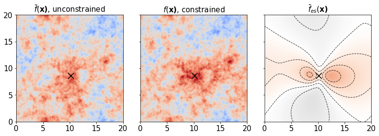
Visualize the constrained density field

Here we plot the unconstrained, constrained density fields and the ensemble mean field, projected on xy plane with slab width of 5 Mpc/h to better visualize the surrounding of the peak.

f, axes = plt.subplots(1,3,sharex=True,sharey = True,figsize=[13,4])
f.subplots_adjust(hspace=0.15,wspace=0.15)
cms = ['coolwarm','coolwarm','RdGy_r']
titles = [r'$\tilde{f}(\bf{x})$, unconstrained',r'$f(\bf{x})$, constrained',r'$\bar{f}_{es} (\bf x)$']
for i,dx in enumerate([dx_field,dx_constraint,dx_ensemble]):
    ax = axes.flat[i]
    projection = np.transpose(np.mean(dx[:,:,70:102],axis=-1))
    ax.imshow(projection,cmap=cms[i],origin='lower',vmin=-10,vmax=10,extent=(0,Lbox,0,Lbox))
    ax.scatter(xpk[0],xpk[1],s=150,marker='x',c='black')
    ax.set_title(titles[i],fontsize=15)
    if i==2:
        ax.contour(projection,colors='black',alpha=0.8,linewidths=1,linestyles='dashed',levels=5,extent=(0,Lbox,0,Lbox))

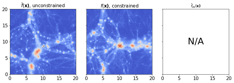
Now we evolve unconstrained, constrained density fields with a non-linear model, projected on xy plane with slab width of 5 Mpc/h.

This may take about 1 minute – but look, the largest halo has shifted to the peak of the constraint!

Q = solver.pm.generate_uniform_particle_grid(shift=0.5)

den_field_lin = solver.pm.create('real', value=dx_field)
S = solver.lpt(den_field_lin.r2c(), Q, 0.1, order=2)
S = solver.nbody(S, leapfrog(np.linspace(0.1, 1.0, 10)))
dx_field_nl = solver.pm.paint(S.X)

den_field_lin = solver.pm.create('real', value=dx_constraint)
S = solver.lpt(den_field_lin.r2c(), Q, 0.1, order=2)
S = solver.nbody(S, leapfrog(np.linspace(0.1, 1.0, 10)))
dx_constraint_nl = solver.pm.paint(S.X)

f, axes = plt.subplots(1,3,sharex=True,sharey = True,figsize=[13,4])
f.subplots_adjust(hspace=0.15,wspace=0.15)
Q = solver.pm.generate_uniform_particle_grid(shift=0.5)

ax = axes.flat[2]
ax.set_title(titles[2])
ax.text(0.5, 0.5, 'N/A', fontsize=30, ha='center', va='center', transform=ax.transAxes)

for i,dx_nl in enumerate([dx_field_nl,dx_constraint_nl]):
    ax = axes.flat[i]
    projection = np.log(1 + np.transpose(np.mean(dx_nl[:,:,70:102],axis=-1)))
    ax.imshow(projection,cmap=cms[i],origin='lower', vmin=0, vmax=6, extent=(0,Lbox,0,Lbox))
    ax.scatter(xpk[0],xpk[1],s=150,marker='x',c='black', alpha=0.3)
    ax.set_title(titles[i],fontsize=15)